In addition to the lack of high-level semantic representations, the sampling of positive and negative samples for instance discrimination tasks also has obvious problems. Positive samples are all from its own data augmentation, while negative samples are directly sampled from a large memory (within the same batch, memory bank or a momentum encoder). The problem with this is that negative samples may have positive sample, which they are the same class, but are different instances. Another problem is that hard negative samples and easy negative samples have the same weights in InfoNCE loss , which make model too simple if it focus on too many easy negative samples. In this chapter, we will see many interesting works with different methods on solving sampling problem in CL.
What Should Not Be Contrastive In Contrastive Learning
Link: https://arxiv.org/abs/2008.05659
Motivation:
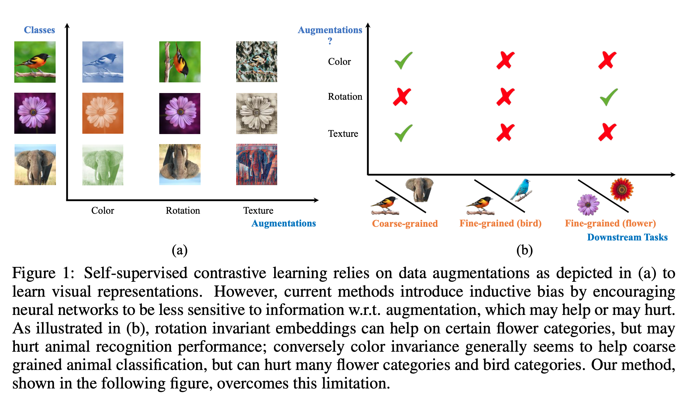
This paper proposed that data augmentation may hurt image representations, especially when they are used on downstream tasks. For example, representation vectors by color augmentation are used on a bird identification task , or representation vectors by rotation augmentation are used on a animal identifacation task.
Sounds reasonable, and it did!
Result:
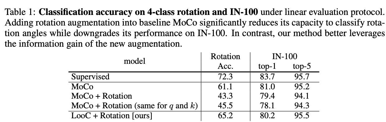
Table 1 shows that add rotation augmentation on MoCo will significantly reduces its accuracy on IN-100(ImageNet-100) this dataset. And their model LooC has a better result.
Method:
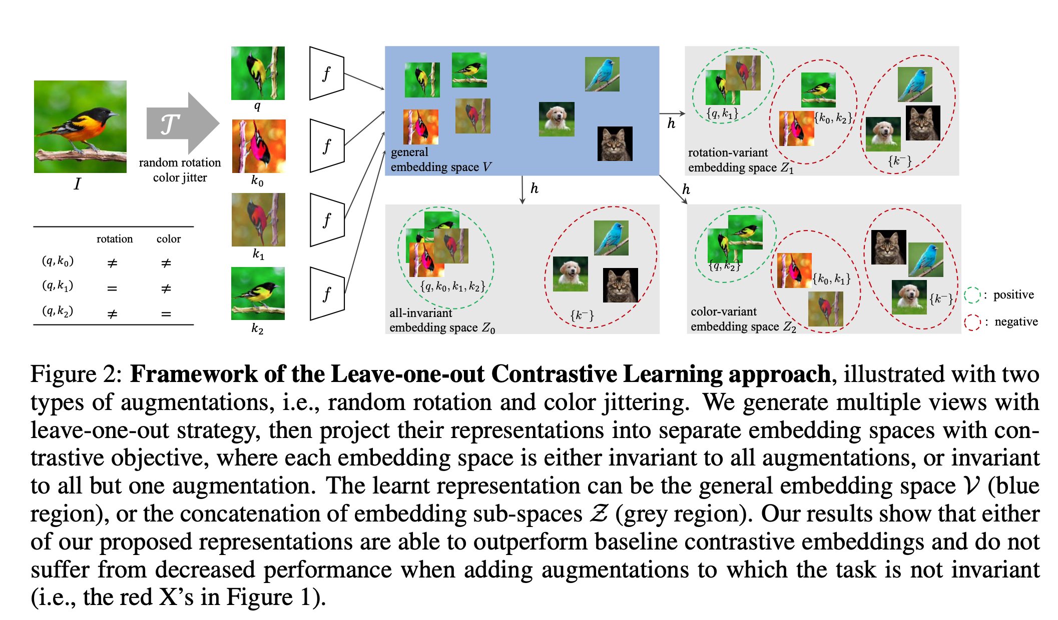
And add all these \(Z\) regions into loss function:
\[\mathcal{L}_{q}=-\frac{1}{n+1}\left(\log \frac{E_{0,0}^{+}}{E_{0,0}^{+}+\sum_{k^{-}} E_{0,0}^{-}}+\sum_{i=1}^{n} \log \frac{E_{i, i}^{+}}{\sum_{j=0}^{n} E_{i, j}^{+}+\sum_{k^{-}} E_{i, i}^{-}}\right)\]
where \(E_{i, j}^{\{+,-\}}=\exp \left(\boldsymbol{z}_{i}^{q} \cdot \boldsymbol{z}_{i}^{k_{j}^{\{+,-\}}} / \tau\right)\)
Insights:
I think the movitation is quite reasonable. But actually, I am not clear about the method and this paper do not provide pesudo code or open source code. I am not sure that if aggregating all different augmentation infomations into the same loss function will solve the problem of different specific downstream tasks. It's more like an improvement in robustness, rather than aiming at adapting with specific downstream tasks.
Boosting Contrastive Self-Supervised Learning with False Negative Cancellation
Link: https://arxiv.org/abs/2010.02037
Motivation:
Negative samples by instance discrimination will contain many potential positive samples(images in the same class). And these false negative samples will hurt CL in 2 ways: discarding semantic information and slow convergence
Method:
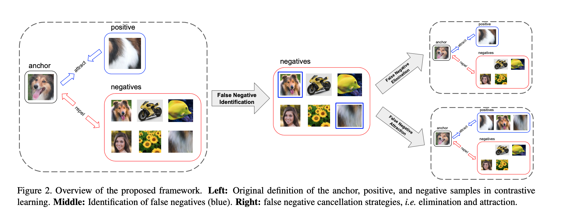
There are 3 parts:
- Traditional CL framework
- False Negative Identification
- False Negative Cancellation
- Elimination
- Attraction
The first part is the model backbone. This paper use SimCLR and MoCo.
The second part is the method how to find those false negatives without label information.
The approach to identify false negatives based on the following observations:
- False negatives are samples from different images with the same semantic content, therefore they should hold certain similarity (e.g., dog features).
- A false negative may not be as similar to the anchor as it is to other augmentations of the same image, as each augmentation only holds a specific view of the object
Based on above observations, the strategy follows as:
- Create a support set contains the image itself, its original augmentation(put into model), and extra augmentations (to hold the second observation).
- Each negative sample compute a similarity score set, e.g. a negative sample will have 8 similarity scores if the size of support set is 8. This paper use cosine similarity.
- Using an aggregation method for the similarity score set, Maximum or Mean
- Selecting the most similar negative samples as false negative samples.
- Select top k high similarity samples
- Select the samples those similarity score is greater than a threshold
The third part is how to use these false negative samples. There are 2 approaches:
False Negative Elimination: These false negatives do not contrast against them, which means drop them from the loss function.
False Negative Attraction: These false negatives will be added into positive samples just like supervised contrastive learning’s loss function.
Insights:
This paper gives many insights from their exhaustive experiments since it is from Google.
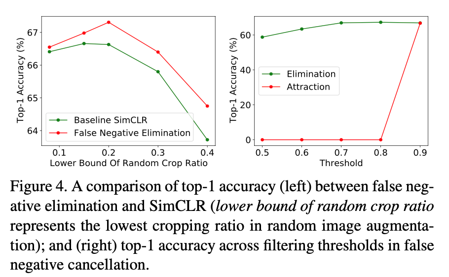
The Gap between FNE and baseline will be larger with the increasing random crop ratio. It is reasonable since larger crop ratio will lead to a higher ratio of false negatives.
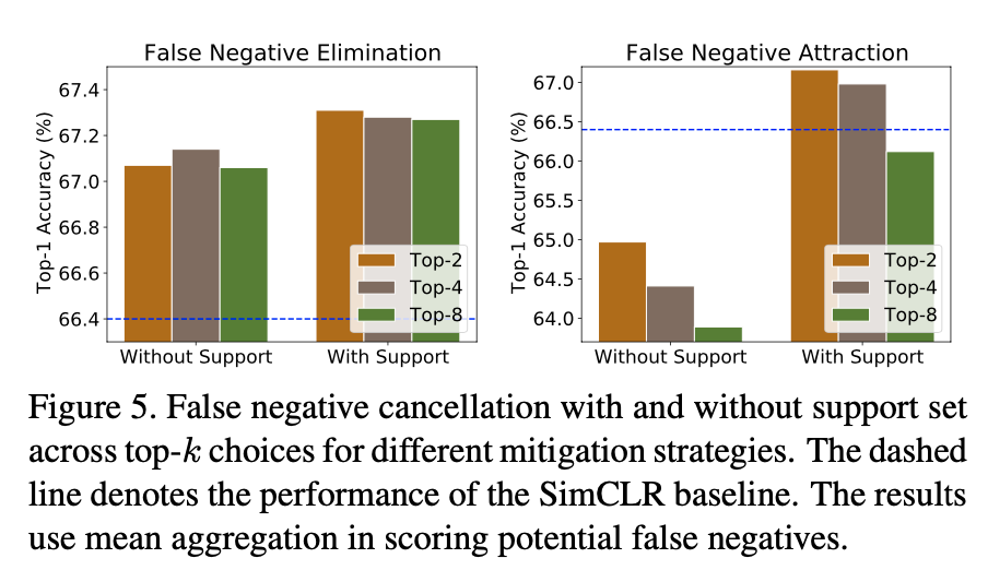
The attraction strategy is much more sensitive to the quality of the found false negatives compared to the elimination strategy.
The paper has many other interesting findins and really recommend you to read paper.
Unsupervised Representation Learning by Invariance Propagation
Link: https://arxiv.org/abs/2010.11694
Motivation:
This paper also aims to solve the positive/negative sampling problem.
- negative samples by random may have positive samples.
- Positive samples also should have different levels. Easy positive samples and hard positive samples have the same impact on model now.
Method:
This paper has a assumption that:
If two points v1 and v2 in a high-density region are close, then their semantic information should be similar.
Hence, we can use metric method like KNN to calculate anchors’ positive samples step by step.
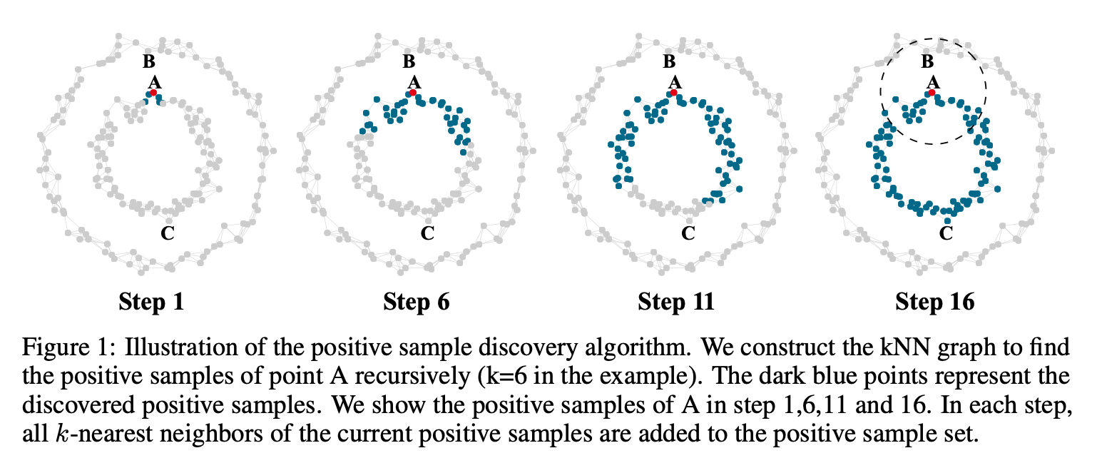
Strategy of Positive samples of an anchor image:
The process is illustrated in Fig 1. In each step, all k-nearest neighbors of the current discovered positive samples are added to the positive sample set. The process repeats l steps.
The difference between tradition KNN and their approach can be shown in the last step of Figure 1. Samples in the dashed circle are positive samples discovered by KNN. By comparison, in their approach, point B is included in K-nearest neighbors of point A and point C is not included.
Hard Sampleing Strategy:
The core is that this paper think positive samples which are already close to the anchor and negative samples which are already far away from the anchor are easy samples. They do not need to be optimized more. However, those positive samples that are far away in the positive sample set(C in Fig 1 )and the negative samples that are relatively close(B in Fig 1) are difficult samples that are more helpful to the model.
Strategy:
Select P samples with the lowest similarity to construct the hard positive sample set \(\mathcal{N}^{h}(i)\).
These hard positive samples deviate far from the anchor sample such that they provide more intra-class variations, which is beneficial to learn more abstract invariance.
Denote the M nearest neighbors of \(v_i\) as \(\mathcal{N}_{M}(i)\), The \(M\) is large enough such that \(\mathcal{N}(i) \subseteq \mathcal{N}_{M}(i)\). Then denote the hard negative sample set \(\mathcal{N}_{n e g}(i)=\mathcal{N}_{M}(i)-\mathcal{N}(i)\).
Then the hard sample mining loss can be like:
\[\begin{aligned} \mathcal{L}_{i n v}\left(x_{i}\right) &=-\log P_{v_{i}}\left(\mathcal{N}^{h}(i) \mid B(i)\right) \\ &=-\log \frac{\sum_{p \in \mathcal{N}^{h}(i)} \exp \left(\bar{v}_{p} \cdot v_{i} / \tau\right)}{\sum_{n \in B(i)} \exp \left(\bar{v}_{n} \cdot v_{i} / \tau\right)} \end{aligned}\]
The overall loss function is just InfoNCE + hard sample mining loss, as follow:
\[\mathcal{L}\left(x_{i}\right)=\mathcal{L}_{i n s}\left(x_{i}\right)+\lambda_{i n v} \cdot \omega(t) \cdot \mathcal{L}_{i n v}\left(x_{i}\right)\]
where \(\omega(t)\) as 0 is the first T epochs, because it is not reliable in frist \(t\) epoches.
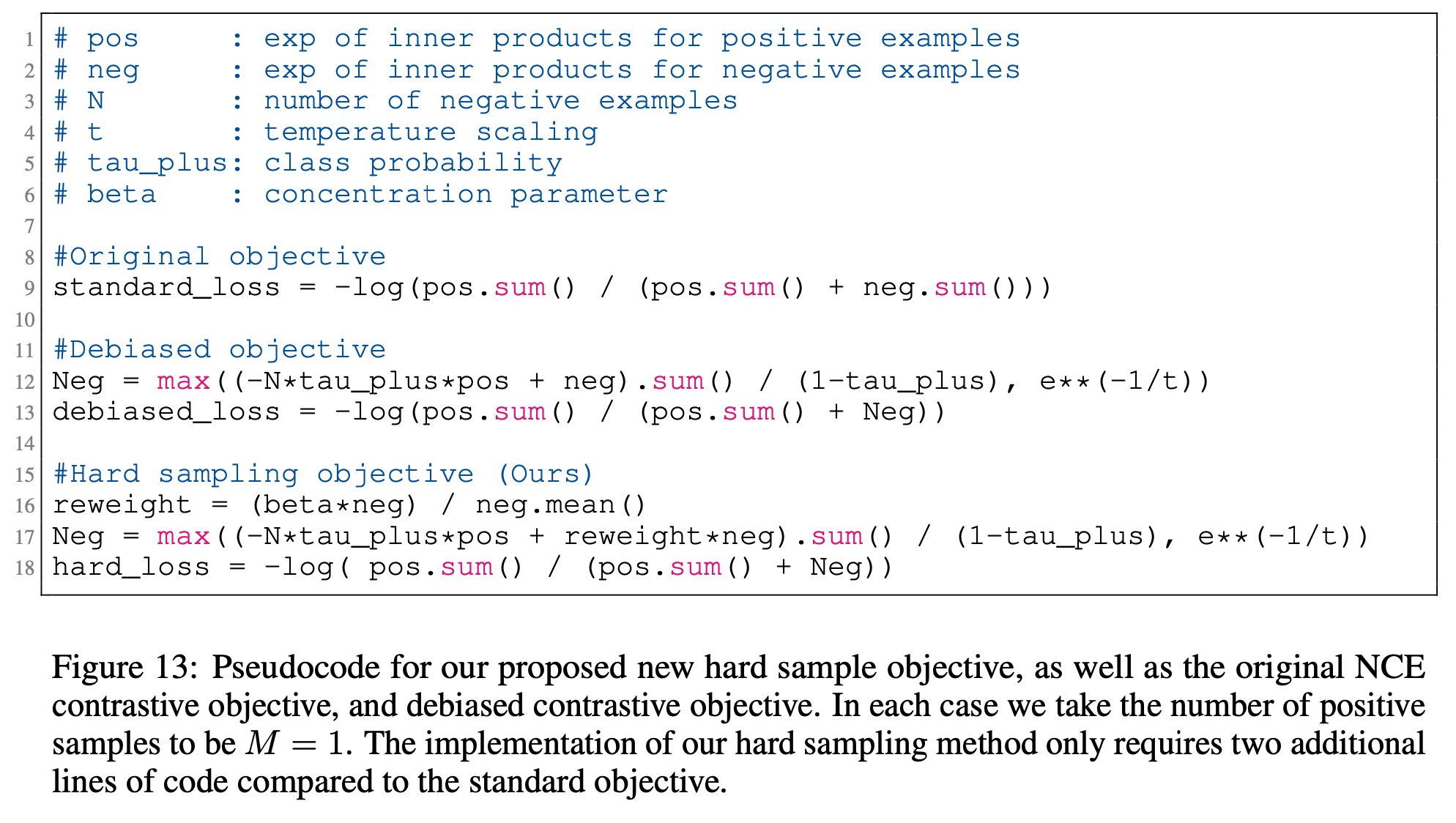
Contrastive Learning With Hard Negative Samples
Link: https://arxiv.org/abs/2010.04592
Motivation:
This paper also focus on negative samples. In metric learning, some work proves that hard negative samples can help guide a learning method to correct its mistakes more quickly (Schroff et al., 2015; Song et al., 2016). Therefore, this paper also wants to use hard negative samples in contrastive learning. Compared with metric learning, contrasitive learning is a unsupervised task, so there are 2 challenges:
- We do not have access to any true similarity of dissimilarity information.
- We need an efficient sampling strategy for this tunable distribution.
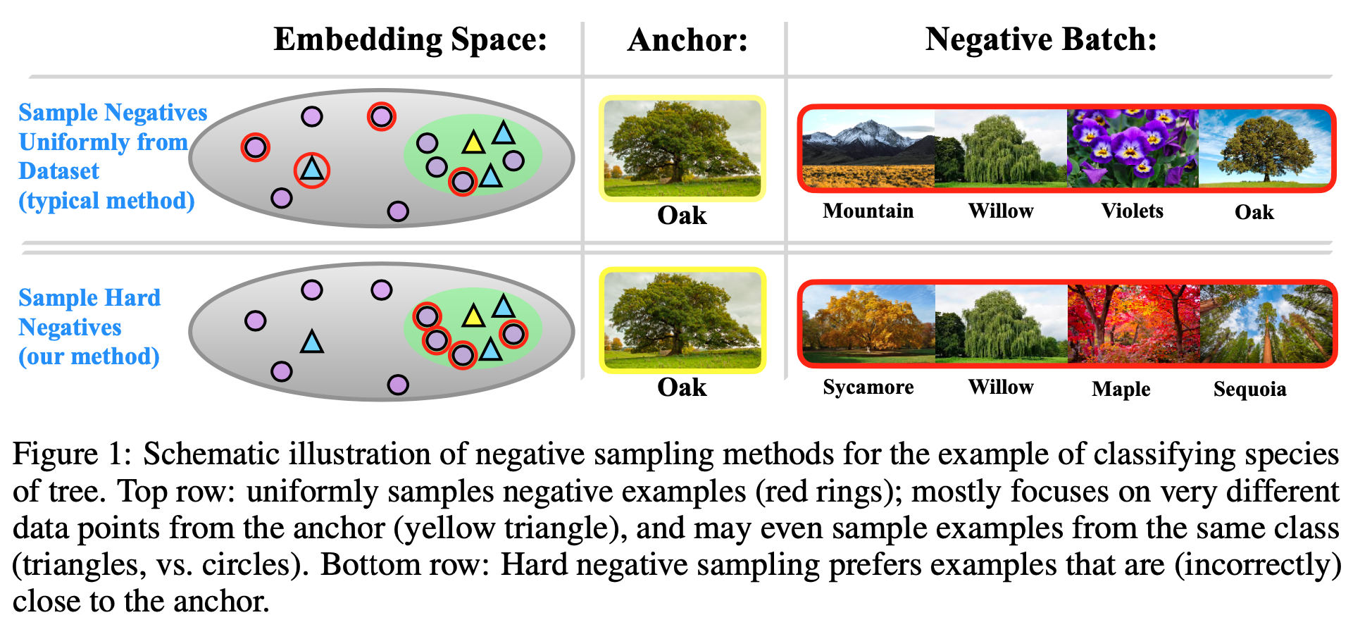
This paper use Figure 1 to show the defination of Hard Negatives.
Method:
We begin by asking what makes a good negative sample?
To answer this question we adopt the following two guiding principles:
Principle 1. q should only sample “true negatives” \(x_i\) whose labels differ from that of the anchor x.
Principle 2. The most useful negative samples are ones that the embedding currently believes to be similar to the anchor.
Because of no supervision, upholding Principle 1 is impossible to do exactly. This paper aims to upholds Principle 1 approximately, and simultaneously combines this idea with the key additional conceptual ingredient of “hardness” (encapsulated in Principle 2).
The theory of this article is very solid with lots of mathmatical prooves, which I want to skip them and only give the final loss pesudo code.
Insights:
I think that the core of this paper is that they think negative samples those are not very close to and also are not too far from the anchor in the encoding space(called Hard negative samples) are useful for model to learn better representation.
Hence, I think it is similar with the previous paper: find those ture negative samples without prior knowledge, where the difference is on different statistics methods.
Hard Negative Mixing for Contrastive Learning
Link: https://arxiv.org/abs/2010.01028
Conditional Negative Sampling For Contrastive Learning of Visual Representations
Link: https://arxiv.org/abs/2010.02037
Debiased Contrastive Learning
Link: https://arxiv.org/abs/2007.00224
Contrastive Crop
Link: https://arxiv.org/abs/2202.03278
Github: https://github.com/xyupeng/ContrastiveCrop
Motivation:
Random crop will hurt image and decrease image semantic.
A method for sampling true right positive samples.
提出了一种技术,
从图中可以发现,对比学习模型本身就可以捕捉物体大概的位置信息,从而来指导crops的选取。
利用这种特征提取物体边框,避免错误正样本对
中心抑制,上述方法由于其带来了更小的选取范围,生成具有较高相似度的样本对的可能性也提高了
降低crops集中在图片中心的概率,从而增大采样的方差。
Conclusion
So far, we have seen a lot of works on how to sample more accurate and better quality positive/negative samples without labels.
Use similarity metrics by images’ embedding vectors to get more reliable samples based on the assumption that same class embedding will be close/similar in the hyperplane.
Restrict data augmentations to achieve more reliable samples by Contrastive Crop or LooC.
So can we combine these 2 ideas that using similarity metrics of the anchor and its augs to sort positive samples with data augmentations as true positive samples and low similarity augs as true negative samples even they are augmentations from the same image.